Simple Bézier Curves in Matlab (2013-11-17)

I’ve always been curious about how [Bézier] cubic splines are generated and I how I can use them in various projects (game development probably being the most immediately obvious). If you don’t know what I’m talking about, Wikipedia has a decent if somewhat tedious description. After digging through the math, I came up with these results which I’ll share for the simplicity of it all (they really are simpler than I ever though). I found most sources started at the beginning and gave huge mathematical backgrounds, which although are nice, are typically just not what I was looking for. What I was looking for (and what is presented here) is just the end result—given a set of input weights, how do I calculate the actual spline?

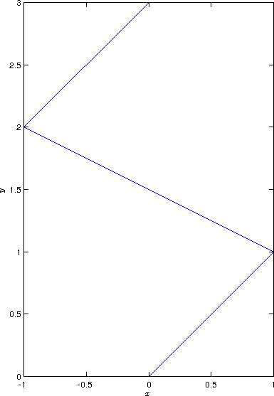
First things first, this is the kind of spline I’m talking about:

Bézier splines are parametric curves, meaning instead of a function like:

y(x) = ...

you instead get functions like:

\begin{aligned} x(t) &= \ldots \\\\ y(t) &= \ldots \end{aligned}

Where $t \in [0, 1]$ . This isn’t a big deal though, and in fact makes our lives even easier—we can just create a list of points in between 0 and 1 and get the corresponding x, y, [and z] coordinates that belong there:

t = linspace(0, 1);

The next thing we need to know is that $x(t)$ and $y(t)$ are just polynomials, defined as:

\begin{aligned} x(t) &= At^3 + Bt^2 + Ct + D \\\\ y(t) &= Et^3 + Ft^2 + Gt + H \end{aligned}

Where $A \ldots H$ are just coefficients. These coefficients can be calculated as such:

\begin{bmatrix} A \\\\ B \\\\ C \\\\ D \end{bmatrix} = \begin{bmatrix} -1 & 3 & -3 & 1 \\\\ 3 & -6 & 3 & 0 \\\\ -3 & 3 & 0 & 0 \\\\ 1 & 0 & 0 & 0 \end{bmatrix} \begin{bmatrix} x_0 \\\\ x_1 \\\\ x_2 \\\\ x_3 \end{bmatrix}

and:

\begin{bmatrix} E \\\\ F \\\\ G \\\\ H \end{bmatrix} = \begin{bmatrix} -1 & 3 & -3 & 1 \\\\ 3 & -6 & 3 & 0 \\\\ -3 & 3 & 0 & 0 \\\\ 1 & 0 & 0 & 0 \end{bmatrix} \begin{bmatrix} y_0 \\\\ y_1 \\\\ y_2 \\\\ y_3 \end{bmatrix}

Or, if you’re not big into matrices and vectors:

\begin{aligned} A &= x_3 - 3 x_2 + 3 x_1 - x_0 \\\\ B &= 3 x_2 - 6 x_1 + 3 x_0 \\\\ C &= 3 x_1 - 3 x_0 \\\\ D &= x_0 \end{aligned}

Note that the equations are essentially the same for each dimension, so $z$ would follow the exact same format (note how the $y$ coefficients are calculated the exact same way as the $x$ ones).

In order to construct this in Matlab, we could do something like the following:

x = [0; 1; -1; 0];
y = [0; 1; 2; 3];

Such that we get points like:

We can then calculate coefficients as such:

C = [-1, 3, -3, 1; 3, -6, 3, 0; -3, 3, 0, 0; 1, 0, 0, 0];
Cx = C * x; % Cx = [6; -9; 3; 0]
Cy = C * y; % Cy = [0; 0; 3; 0]

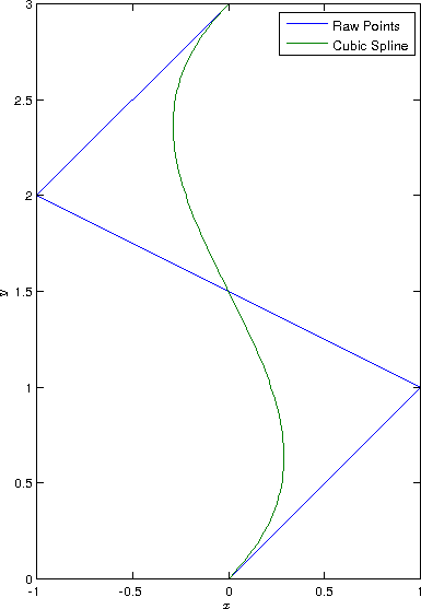
Finally, to create the parametric curve we can combine everything:

sx = polyval(Cx, t);
sy = polyval(Cy, t);
plot(sx, sy);

So that we get something like:

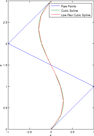
The cubic spline using the given raw points

Note that the “resolution” of this is entirely dependent on the number of points that exist in t. By default, in linspace, this will be 100, but we can easily drop that down:

t = linspace(0, 1, 10);
sx = polyval(Cx, t);
sy = polyval(Cy, t);
plot(x, y, sx, sy);

Which results in:

We can reduce the resolution of the spline substantially and still get decent results

And we’re done! That was a lot easier than I was expecting!

Note that this formulation is just for one segment that would typically be part of a much longer line composed of multiple segments. If we wanted to connect two segments together, in order to make the connection smooth all we have to do is ensure the slope of these curves are equal. The easiest way to do this would most likely be to calculate $(x_1, y_1)$ in the second segment using $(x_2, y_2)$ and $(x_3, y_3)$ from the first segment such that:

\begin{aligned} x_0^2 &= x_3^1 \\\\ x_1^2 &= \left(x_3^1 - x_2^1\right) + x_3^1 \\\\ &= 2x_3^1 - x_2^1 \\\\ \end{aligned}

(Use the same formulation for the $y$ dimension).

I’ll probably post more things later, such as how to calculate the length of each spline segment so that we can do things like determine appropriate $t$ resolutions and calculate total lengths of lines etc, but hopefully this will get you off to a start right now!